Update: Third article is here, Continual Learning with Marketplace: Model Learns New Data with Mostly Inference
Two weeks ago, I published an article, Marketplace: My first attempt at training without backprop on GPU efficiently. To my surprise, it received far more positive feedback than I expected. I was thrilled that people found my research project interesting, and I greatly appreciate the kind words from readers.
Curious about how far I could push this idea, I spent another two weeks improving it. Initially, my research focused on enhancing the scalability of the Marketplace algorithm. I implemented seed-based random number generation for each vendor’s weights, as mentioned in the previous article. I also explored other ideas to improve the Marketplace algorithm, such as using a second forward pass to determine the optimal learning rate. However, exploring permutations of the loss outputs to compose a better overall delta, accounting for both good and bad outcomes, truly blew my mind 🤯.
The performance is now on par with backpropagation in certain configurations. Here’s the comparison with backpropagation plus Stochastic Gradient Descent (SGD) as the optimizer:

A diagram with 50% smoothing shows the comparison of the validation accuracy between the Marketplace V2, V1 algorithms and the backprop with SGD as the optimizer based on different learning rates. The Marketplace V2 algorithm outperforms the Marketplace V1 algorithm greatly and the backprop with SGD as the optimizer at 1e-3 learning rate. It only lose to the backprop with SGD as the optimizer at 3e-3 learning rate and 7e-3 learning rate. While backprop with SGD as the optimizer is still better, but I believe with hyperparameter tuning, the Marketplace V2 algorithm can at least match it.

A diagram with 50% smoothing shows the comparison of the loss between the Marketplace V2, V1 algorithms and the backprop with SGD as the optimizer based on different learning rates. The Marketplace V2 algorithm outperforms the Marketplace V1 algorithm greatly and the backprop with SGD as the optimizer at 1e-3 learning rate and 3e-3 learning rate in later steps. It only lose to the backprop with SGD as the optimizer at 7e-3 learning rate. While backprop with SGD as the optimizer is still better, but I believe with hyperparameter tuning, the Marketplace V2 algorithm can at least match it.
I believe my research has a significant potential to revolutionize the machine learning training process. Today, I’m excited to share the improvements to the Marketplace algorithm, which I call the Marketplace V2 algorithm.
Why Does Marketplace Work?
In my last article, I explained how it works. However, I didn’t delve into why it works. After publishing, I reflected on this question because understanding why it works is crucial for improving the algorithm, otherwise, I’d be left guessing and testing. While I haven’t had time to test these hypotheses, here’s my reasoning.
When discussing gradient descent, people often compare it to walking down a hill. This analogy isn’t entirely accurate because the terrain appears to change when you mutate parameters, as noted in this video.

A screenshot of a video titled "The Misconception that Almost Stopped AI," explaining that the terrain changes when parameters are mutated.
Despite it may not be 100% accurate, this analogy provides a good intuition for gradient descent.

A diagram of a curve with an arrow pointing in the direction of the steepest descent.
With backpropagation, we measure the slope of the terrain and descend carefully. But do we really need such precision? The Marketplace algorithm, instead of measuring the slope, feels more like sending probes in random directions and selecting the best one.

A diagram of probes sent in random directions to find the best one.
The algorithm’s clever trick is reusing intermediate products to efficiently create more permutations of the probe candidates.

A diagram showing more colored probes in random directions than the previous diagram. We reuse intermediate products to create more permutations of the best probe efficiently.
The more probes you send, the higher the chance of finding good ones, some of which will roughly move in the right direction. With a large model, the number of parameters creates a vast search space. But are all parameters equally important? The lottery ticket hypothesis suggests that only a small subset of parameters are critical.
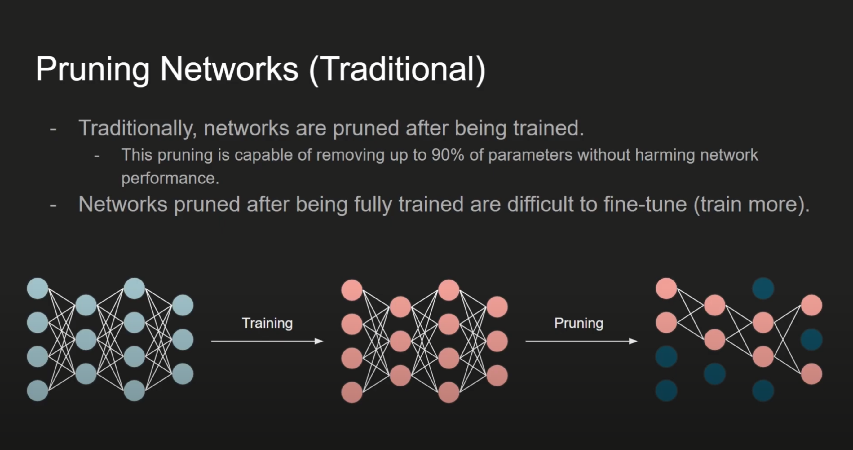
A screenshot of a video about the lottery ticket hypothesis.
Thus, for probes to trend in the right direction, only a small subset of parameters needs to align correctly. Most parameters are likely just noise. As long as a probe’s overall direction has more upside than downside, it’s good enough.

A diagram showing that probes (delta) may contain positive and negative changes, but as long as the upside outweighs the downside, the probe is good enough.
The Marketplace algorithm selects the best combination of parameters from the probes. Since the leading vendor for each specification remains unchanged, it only mutates if the new direction is slightly better. This process accumulates small, fortunate changes over time, eventually leading to a good solution.
The Problem with Marketplace
As mentioned in the previous article, the Marketplace algorithm selects only the best parameter combination from the probes, discarding all others. “Best” refers to the combination with the lowest loss. While this combination reduces overall loss, it’s an all-or-nothing approach. By accepting the best probes, we also incorporate mutations that may increase loss in some aspects.
This is wasteful because other combinations also provide valuable directional information. The best probes have more beneficial mutations than harmful ones, which is why they’re selected. However, as parameters improve, finding better mutations becomes harder, and the probability of good mutations decreases compared to bad ones. At that point, more probes are needed to find a good mutation.
Let’s view the Marketplace algorithm through the lens of a real-world marketplace. When a product sells well, multiple factors contribute to its success. The same applies to factors causing poor performance. For a vendor, many parameters influence the product, making it hard to pinpoint the most critical one. But what if you have enough products with slightly adjusted parameter permutations? Couldn’t you statistically attribute the product’s performance to the parameter adjustments? Yes! That’s the core idea behind the Marketplace V2 algorithm.
The V2 Algorithm
The V2 algorithm is largely similar to the V1 algorithm, except that we reward each parameter delta based on the performance of the final product and compose the overall delta from the delta of each parameter. Please read the first article for the details of the V1 algorithm. Here’s how it works:
There are combinations of loss and their corresponding paths. Let’s say each loss is \(L_i\), the parameter is \(\theta\), and the corresponding delta is \(\Delta \theta_i\), where \(i\) is the index of each unique path. The mean loss is:
\[\mu = \frac{1}{n} \sum_{i=1}^{n} L_i\]The standard deviation of the loss is:
\[\sigma = \sqrt{\frac{1}{n} \sum_{i=1}^{n} (L_i - \mu)^2}\]We normalize the loss by subtracting the mean value and dividing by the standard deviation. We call this attribution and denote it as \(A_i\):
\[A_i = - \frac{L_i - \mu}{\sigma}\]Note that we invert the sign because we want to reward parameter deltas that contribute to a lower loss and penalize those that contribute to a higher loss.

A diagram showing the conversion of the loss of each final product, calculation of attribution by normalizing the loss, and flipping the sign.
Then, we attribute the loss to the parameter delta that contributed to it:
\[\Delta R = \sum_{i=1}^{n} A_i \times \Delta \theta_i\]We call \(\Delta R\) the reconciled delta because it accounts for the performance of the final product for each parameter. It’s like distributing the profit or loss to the parameter deltas that contributed to it.
To calculate the reconciled delta, the process is straightforward. We take the attribution value \(A_i\) and multiply it by the parameter delta \(\Delta \theta_i\) for each unique path, i.e., the vendors’ deltas on each path.

A diagram showing multiplication of the attribution value with the parameter delta of vendors at a unique path.

A diagram showing multiplication of the attribution value with the parameter delta of vendors at a different unique path.
Finally, we sum the delta multiplied by the attribution value for each unique path:

A diagram showing the summation of the delta multiplied by the attribution value for each unique path.
The reconciled delta \(\Delta R\) is a vector pointing in the direction that leads to better overall performance. We believe this is somewhat similar to the gradient direction in backpropagation. The reconciled delta should approximate the gradient direction in backpropagation, and with more samples, the direction should converge closer to the true gradient direction.
From a linear algebra perspective, we are essentially composing a linear combination of the parameter deltas at each path. For the direction that is most correct, we assign more weight to the parameter delta at that path. For those pointing in the wrong direction, we assign a negative weight to the parameter delta to redirect it toward the correct direction. For neutral directions, we assign weight close to zero to the parameter delta to avoid affecting the overall direction.

A diagram showing attribution of the loss to the parameter delta vector at each path.
Since the directions are random, unrelated parameters in the vectors should cancel each other out. A bad direction is also helpful in finding the right direction because we multiply it by a negative weight, effectively pointing it toward the correct direction.

A diagram showing that the combined vector approximates the gradient direction in backpropagation.
As the scale of the reconciled delta may not be appropriate, we normalize it to a unit vector:
\[\Delta G = \frac{\Delta R}{||\Delta R||}\]We believe this unit vector direction is nearly identical to the gradient direction in backpropagation, so we call it the gradient direction and denote it as \(\Delta G\). With the gradient direction \(\Delta G\), you can update the parameters by multiplying it by the learning rate \(\eta\):
\[\theta' = \theta + \Delta G \times \eta\]The next is basically updating the seeds and generate random small weight deltas based on the seeds for each vendor, and then repeat the process.
Comparison with Backprop
In the previous article, I forgot to mention that the backprop experiment uses Adam as the optimizer. I realized it’s somewhat unfair to compare the Marketplace approach with backprop because I was not only competing against backprop but also the Adam optimizer. The backprop algorithm is highly performant, and Adam enhances its power. I heard some people said that Adam is the optimizer on steroids, well, using steroid in a fight is obvious cheating, right? In contrast, the Marketplace algorithm simply applies a learning rate to the gradient direction, which is essentially equivalent to SGD. Therefore, it makes more sense to compare the Marketplace algorithm with backprop using SGD as the optimizer.
Please note that in the previous article, we swapped the Batch Normalization layer for an Instance Normalization layer in the backprop algorithm. However, when running backprop with SGD as the optimizer, we reverted to the Batch Normalization layer because the Instance Normalization layer does not perform well with SGD for this particular model. For the Marketplace algorithm, we kept the Instance Normalization layer, as the Batch Normalization layer is less effective with this approach.
With a more level playing field, the results are much more exciting. I observed very similar performance between the Marketplace V2 algorithm and backprop with SGD as the optimizer. Here are the results:
A diagram with 50% smoothing showing the comparison of validation accuracy between the Marketplace V2, V1 algorithms, and backprop with SGD as the optimizer across different learning rates. The Marketplace V2 algorithm significantly outperforms the Marketplace V1 algorithm and backprop with SGD at a 1e-3 learning rate. It only falls behind backprop with SGD at 7e-3 and 3e-3 learning rates.
A diagram with 50% smoothing showing the comparison of loss between the Marketplace V2, V1 algorithms, and backprop with SGD as the optimizer across different learning rates. The Marketplace V2 algorithm significantly outperforms the Marketplace V1 algorithm and backprop with SGD at a 1e-3 learning rate. It only falls behind backprop with SGD at a 7e-3 learning rate.
Both Marketplace algorithms use the same market depth and vendor count: a market depth of 3 and 16 vendors per specification.
Certainly, with the right learning rate, backprop with SGD as the optimizer still outperforms the Marketplace V2 algorithm. However, this is already very exciting! Unlike backprop, which requires both forward and backward passes, the Marketplace algorithm only needs the forward pass. I haven’t spent much time on hyperparameter tuning for the Marketplace V2 algorithm because, with 16 vendors, the startup time for Tinygrad is lengthy due to its JIT compiler compiling kernel code for very complex compute graph, slowing down the hyperparameter tuning process (the new rangify feature could potentially solve this, but it’s not yet stable). The fact that the Marketplace V2 algorithm shows nearly identical performance at certain learning rates suggests that this is likely a hyperparameter tuning issue.
The Marketplace V2 algorithm is still new, and we are unsure how to optimally tune its hyperparameters to further improve performance. However, I believe it’s only a matter of time before we find the right hyperparameters or optimize the algorithm itself to match or exceed the performance of backprop with SGD. We can also scale the Marketplace V2 algorithm with more vendors and depth if a more accurate gradient direction is needed. Additionally, I’ve experimented with techniques like using a second forward pass to adjust the learning rate, which shows promising results but requires further refinement. Because it only requires a forward pass, the Marketplace V2 algorithm could, in theory, run at least twice as fast as backprop. With these considerations, I assert that the Marketplace V2 algorithm is on par with backprop using SGD as the optimizer. With further research and optimization, I firmly believe the Marketplace algorithm will even surpass backprop.
What Are the Implications?
Some may ask: What’s the point of expending additional computational resources to achieve the same performance as backpropagation? As mentioned in the previous article, the Marketplace algorithm relies solely on the forward pass to train the model. Optimizing the forward pass is easier and more beneficial for inference performance than optimizing the backward pass. Since backpropagation requires both forward and backward passes—and even assuming the backward pass takes the same time as the forward pass (though it typically takes much longer)—the Marketplace algorithm, by using only the forward pass, could be at least twice as fast as backpropagation. Additionally, the cache-friendly nature of running only the forward pass could make it even faster in practice. While we may lose some accuracy in the gradient direction, I would argue that gradient direction accuracy offers only marginal benefits to the training process once it passes a certain threshold. The Marketplace algorithm essentially trades gradient direction accuracy for training speed and other advantages.
While the forward pass in the Marketplace algorithm is more computationally intensive, it is designed to be GPU-efficient. With a powerful GPU and highly optimized code, it should perform at least as fast as the forward pass in backprop. We also need to compute the reconciled delta for the Marketplace algorithm, but this is only a small fraction of the forward pass and can be easily parallelized.
The potential of the Marketplace algorithm is immense—running at least twice as fast as backprop is just the tip of the iceberg. Many may not realize that GPUs are only part of the equation in large-scale training. Bandwidth is often the bottleneck. The primary reason large-scale distributed training isn’t conducted on idle consumer-grade GPUs is due to bandwidth limitations. When using GPU clusters for training, network bandwidth is a critical factor.
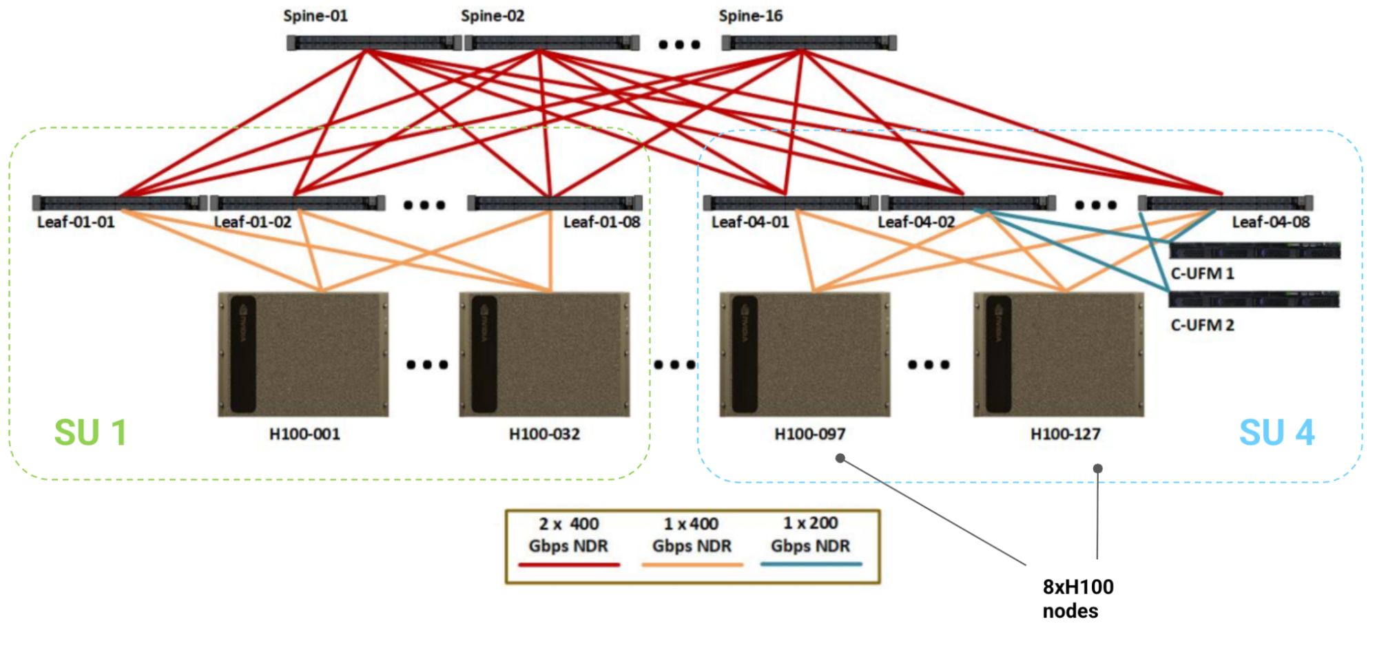
A figure from How to Think About GPUs by Google DeepMind showing the NVIDIA H100 SuperPod architecture, a large-scale GPU cluster. It highlights the tremendously high network bandwidth between nodes, which is critical for large-scale training and expensive to implement.
With the Marketplace algorithm, the bandwidth required for syncing weights is significantly reduced. Using our seed-based random number generation, we only need to redistribute the seeds plus the attribution value \(A_i\) for each path to reconstruct weight updates. This reduction in bandwidth requirements means less time spent syncing weight updates across nodes, which could revolutionize large-scale training. Training time could be significantly reduced. Sorry, Jensen, for the potential impact on NVLink sales! 😅
Due to the reduced bandwidth requirements, I believe this opens up a new world of distributed training. It may become feasible to conduct large-scale training on idle consumer-grade GPUs.
Future Research Directions
The Marketplace V2 algorithm performs comparably to backpropagation, but several questions remain unanswered.
Is Reconciled Delta an Accurate Approximation of the Gradient Direction in Backpropagation?
As noted throughout this article, the reconciled delta performs nearly identically to the gradient direction in backpropagation with stochastic gradient descent (SGD) as the optimizer. This raises the question: Is the reconciled delta an accurate approximation of the gradient direction in backpropagation? To answer this, one could run backpropagation alongside the Marketplace algorithm, compare the gradient direction with the reconciled delta, and evaluate their similarity. Another intriguing question is whether scaling up the Marketplace algorithm could improve the approximation of the gradient direction. Due to time constraints, I leave this exploration to others interested in this topic.
Can We Apply Optimization Techniques to the Marketplace Algorithm?
Assuming the reconciled delta accurately approximates the gradient direction in backpropagation, can we apply optimization techniques such as momentum, Adam, or others to the Marketplace algorithm? If these techniques can be integrated, they could potentially enhance performance with minimal effort.
Scalability of the V2 Algorithm
In my earlier research, I explored the scalability of the Marketplace V1 algorithm, which is relatively straightforward to scale along two main axes:
- The dataset axis: Parallelizing the forward pass.
- The marketplace replication axis: Running multiple marketplace replicas.
Using seed-based random number generation, the Marketplace V1 algorithm can be replicated across multiple nodes and executed in parallel. Due to limited access to GPUs, I simulated this by running multiple forward passes and marketplace replicas sequentially. Increasing the number of forward passes and replicas showed performance improvements on a limited scale, but its effectiveness at a larger scale remains unclear. The V2 algorithm’s scaling behavior differs, so I defer further investigation to future work or others interested in this topic.
Adaptive Learning Rate
I explored the idea of using an adaptive learning rate with the Marketplace algorithm. Since the algorithm allows testing slight parameter changes, it could also test different learning rates. The approach involves using the first forward pass to determine the reconciled delta direction and the second forward pass to identify the optimal learning rate, essentially determining the direction in the first pass and the step size in the second.
Using this second pass to test the learning rate is a promising idea. I implemented this approach, and it significantly improved performance in the initial steps, even outperforming backpropagation with SGD as the optimizer at certain learning rates in the early steps. However, performance degraded later due to fluctuating learning rates.

The validation accuracy of the Marketplace V2 algorithm with an adaptive learning rate outperforms many backpropagation configurations with SGD as the optimizer, using only 8 vendors per specification. However, performance degrades quickly due to fluctuating learning rates.

The loss of the Marketplace V2 algorithm with an adaptive learning rate outperforms many backpropagation configurations with SGD as the optimizer, using only 8 vendors per specification. However, performance degrades quickly due to fluctuating learning rates.
The Marketplace V2 algorithm with an adaptive learning rate shown in the diagrams above uses only 8 vendors per specification, while the one we used in backprop comparsion uses 16 vendors, yet it still outperforms many backpropagation configurations with SGD in early steps. This suggests a promising direction, but stabilizing the learning rate is necessary to prevent performance degradation.
Large Models and Datasets
As discussed in the previous article, I tested the Marketplace algorithm on a larger model like ResNet-18 with a scaled MNIST dataset, but these experiments were insufficient to assess scalability to larger models and datasets. A common saying is:
If it doesn’t work with MNIST, it probably won’t work with anything.
Having demonstrated that the Marketplace algorithm performs well with a small MNIST CNN, the next step is to test it with larger models and datasets. Training larger models and datasets requires significant time and resources for efficient execution, so I defer this to future work or others interested in this topic.
I Need Your Help: Let’s Advance Machine Learning Together
Although I move extremely fast to write code and experiment with new ideas, I still only have 24 hours in a day and 7 days in a week. As you can see, there are so many interesting things to explore with the Marketplace algorithm, and I can only do a small part of it.
As a solo researcher, it’s also scary to think about whether I made mistakes during the process. But I believe the best way to move forward quickly is to embrace mistakes and learn from them rapidly. Maybe it’s a fool’s errand in the end, but I still want to try. People used to believe that training with super-large models was not possible because they would overfit. Until someone brave enough tried it and proved it was possible, which is why we see today’s machine learning blooming. It’s funny that I see countless examples of scientists entering the field where their teachers, professors, or advisors told them everything was well researched and there was nothing new to be found. But we know people have proved that wrong again and again. So the question is not what if I make mistakes, the question is, if we don’t try, how can we know if we can make it? And what if I am right?
If you’re like me and dare to challenge the status quo, I invite you to join me. I believe the Marketplace algorithm is just the beginning of a new era in machine learning. All of my experiments are open-source under the MIT license and accessible to everyone.
https://github.com/LaunchPlatform/marketplace
You can contribute to the project, fork it, and conduct your own research. You’re also very welcome to reproduce the experiments with your own implementation. Please feel free to contact me if you have any questions or suggestions. I am also open to exploring collaboration opportunities if there’s something interesting to pursue together.
Acknowledgments
Many people have mentioned interesting prior works on X. I think it’s helpful to list them here for others to learn from. If you find any interesting prior works somewhat relative to my research, please feel free to let me know, I will add them to the list.
Spike-Timing-Dependent Plasticity
Nathan Odle (@mov_axbx) on X mentioned that my Marketplace algorithm somewhat maps to RL-STDP. It appears that STDP (Spike-timing-dependent plasticity) is a biological process for adjusting the weights of synapses. I haven’t had time to really dig into it, but it’s interesting to see that my Marketplace algorithm could potentially be similar to the biological processes by which the brain learns. By the way, the author’s 7 4090 AI training rack is so cool—be sure to check it out.
Random Feedback Weights Support Learning in Deep Neural Networks
andrew (@gradientjanitor) on X mentioned that my Marketplace algorithm reminds him of another paper: Random feedback weights support learning in deep neural networks by Lillicrap et al. I glanced through the paper and think I understood maybe 50% of the ideas. Regardless, it seems like an interesting paper showing that random feedback weights can support learning in deep neural networks.
Bucket Brigade Algorithm
Sebastian Risi (@risi1979) on X mentioned that it could be somewhat similar to the Bucket Brigade Algorithm by Holland. If we view each vendor on the path to the final product as a chain of actions and the final loss as the reward, it could be somewhat similar to the Bucket Brigade Algorithm. However, there’s no bid and tax in the Marketplace algorithm.
Final Thoughts
Personally, I feel so excited about the future of machine learning and the Marketplace algorithm’s applications. I can’t wait to share one more thing before I end this article. My next research direction is about “continual learning.” In the real world, we learn new things by doing, it’s odd that machine learning requires a dedicated process to learn new things. After I came up with the Marketplace algorithm, I’ve already had the idea of applying it to continual learning. Some people on X also realized the same potential of the Marketplace algorithm before I even announced it.
By continual learning, I mean we can make a model learn new things through inference alone mostly. Sounds exciting, right? I have run the idea through in my mind, and I believe it’s possible. The only thing left is to implement it and see if it really works as I expected. Stay tuned for the upcoming articles. I hope you enjoyed reading this article.