Update: Please read the second article for the details of the V2 algorithm. Also the third article, Continual Learning with Marketplace: Model Learns New Data with Mostly Inference, introduces the continual learning with the Marketplace algorithm.
If you’ve read my previous articles, you know I’m a big fan of first-principles thinking. I’ve mentioned many times that I want to eliminate backpropagation. Many people think I’m crazy and assume I must be joking. But no, I’m serious. I thought about the problem from time to time. Recently, I came up with an idea that could potentially work. I spent two weeks implementing it and running experiments, and it worked! While this is just a baby step, there are still many things to improve, but at least I think it’s an interesting idea that could be worth exploring and sharing. Today, I would like to share my approach to training without backpropagation on GPUs efficiently.

A diagram shows the validation accuracy of a small MNIST CNN model training process without using backpropagation.

A diagram shows the loss of a small MNIST CNN model training process without using backpropagation.
Background
Just because a solution exists and is widely used doesn’t mean it’s the best one. From this perspective, we should challenge all existing solutions. Having worked on numerous machine learning projects recently, I’ve found that backpropagation uses a ton of memory. The dependencies introduced by backward propagation also make it challenging to scale effectively. I want to train a model without backpropagation, ideally in a distributed manner.
I am a very different type of person, I guess. I really don’t like seeing the answer before coming up with my own ideas. This is why I didn’t study any existing research papers or articles about how to train without backpropagation. The interesting thing about research is that one can usually only do so much with existing technologies and methodologies. For example, the concept of the Convolutional Neural Network (CNN) is not new. It was proposed by a Japanese researcher named Fukushima as early as 1979! I saw a post about it on X a few days ago:

CNN history from a X post mentioning that the idea of CNN was introduced long ago by a Japanese researcher, but it only implemented and grains popularity later due to advancements in hardware and training techniques.
At the time the concept was introduced, it would have likely cost the researcher an insane amount of money and resources just to test the idea. The CNN was only proven useful by LeCun et al when backpropagation was introduced and computer resources became more accessible years later.
It’s remarkable to think about: most of our modern-day machine learning methodologies originated decades ago. But things change so fast. While I was studying CUDA, I watched a video entioning that the NVIDIA A100 chip’s computing power surpasses that of a supercomputer cluster, which once took up an entire room, while using only a fraction of the power. It’s insane to think about—I have a 4090 right inside my work PC. It’s a supercomputer in this tiny box! 🤯
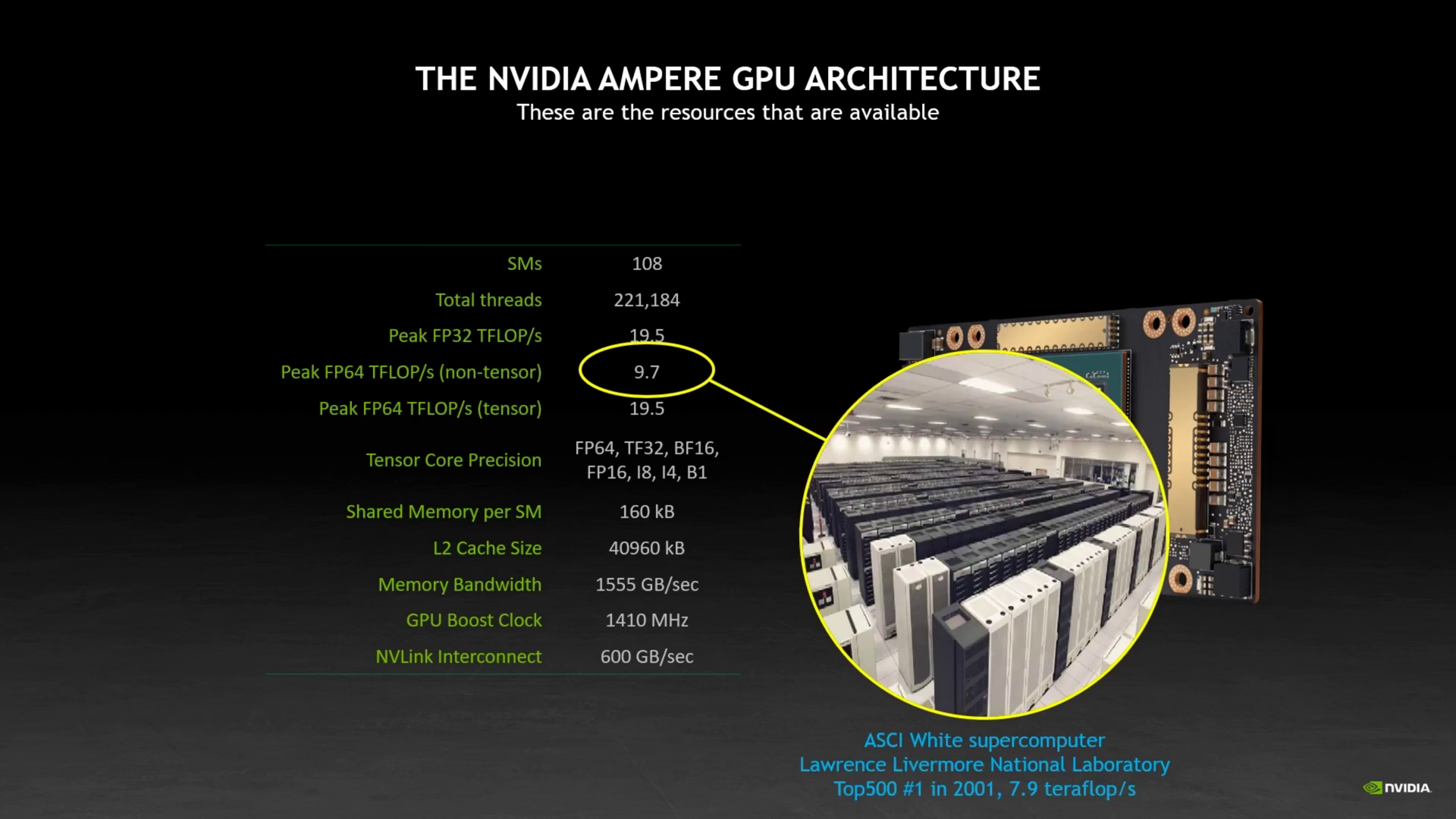
A YouTube video introducing CUDA and how memory access patterns significantly impact CUDA program performance. The video also mentioned that modern GPUs rival the capabilities of supercomputers from a few years ago.
As you can see, given the time and context, it’s hard to imagine how fast future computer chips could become. Even if a researcher could predict what might work, it was prohibitively expensive to test. Most papers are products of the technologies available at their time. That’is why it’s always a good idea to devise solutions from the ground up using today’s technologies.
When I was working on my MAZE project, I thought a lot about how it could be more efficient. The thing is, no matter how interesting your idea is, if it can’t run efficiently with the available resources right now, it’s just science fiction. Sure, I could come up with a system to evolve different models a zillion times to see which one works best, but the problem is that you don’t have the resources to run it a zillion times like Mother Nature does. I saw a presentation by Daniel Han from Unsloth AI, where he mentioned:
Machine learning is all about efficiency
I think that’s true. To make machine learning work, efficiency is key. Great presentation, by the way. If you’re interested in Large Language Models (LLMs), I highly recommend it.
A screenshot of a presentation by Daniel Han from Unsloth AI, where he mentioned that machine learning is all about efficiency.
Take machine learning model mutation, for example. Currently, MAZE can only mutate model structure. But in the real world, I believe model weights could also be encoded in the DNA. Therefore, I’ve been thinking hard about how to mutate not just the structure but also inherit weights from parent models. I realized something really inefficient in my current approach: mutations may only occur at some point in the model structure. For the layers before that mutation, we’ve already fed testing/training data to them previously. So, you’re duplicating work by repeatedly feeding the same data to the same shared layers. One straightforward idea is to cache the values and reuse them, but this may still require a lot of storage space.

A diagram showcasing how mutation only affects downstream layers. With the same input data, we are repeating the same work for the same model.
Since I was also thinking about how to eliminate backpropagation, I wondered if I could apply a similar idea to training.
Idea: Marketplace
Other than Mother Nature, I also like to think about all kinds of efficient organic mechanisms and how they work. A free market is another great example. No matter how the environment changes, a free market can adapt quickly and produce in-demand goods efficiently. I view an entire neural network as a marketplace. Each time data flows into a model, it’s like raw materials acquired by vendors, who then produce products. If you break the model down to a smaller scale, each layer is like a stop in the manufacturing process. When you further break down the layer, each neuron can be seen as a vendor that takes in materials, processes them, and outputs a product to the downstream layers. With this in mind, I’ve been thinking about how to make a neural network model mimic how a free market works. Ideally, each vendor should evolve autonomously and compete to produce the best products.

Comparing a neuron network to a vendor in a marketplace. They both take in materials, process them, and output a product.
Sure, it’s easier said than done. As mentioned previously, machine learning is all about efficiency. I needed to think hard about how to make it GPU-friendly. I tried a few different approaches and finally found something that works efficiently on a GPU. Because the idea is inspired by how a free market works, I call it the “Marketplace.” Here’s how it works.
In a neural network, there are usually many layers. Take a Convolutional Neural Network (CNN), for example: one image could flow through multiple layers of kernels to capture features at different hierarchical levels. The further down the layers, the more abstract the concepts it captures. For each layer, the output is a tensor with the same shape, regardless of the input data. Therefore, I call this a spec. You can think of it as a specification for a product. In each layer, or a group of layers, for a specific set of weight values, I call it a vendor. Think about it: vendors take input, transform it deterministically based on their weights, and output the result as their product. Indeed, they are vendors.

A diagram showcasing that you can think of a layer in a neural network as a specification for a product. Because they all take input in the same shape and output in the same shape.
The idea is to have many vendors in a layer compete to produce the best product for the downstream layers. But here’s the problem: what does the “best” product mean? Before the final end-user evaluates it, nobody knows whether these intermediate products are good or bad. It’s hard to determine how well a product performs if we adjust it slightly. The only way to know is to let the downstream vendors consume it, produce their own products, and eventually have those consumed by the end customers, who provide their feedback.
But then another problem arises. When a vendor in a hidden layer changes their formula slightly, the altered output impacts the products downstream. It’s hard to predict whether a slight increase in the “sweetness” of your sugar supply might ruin the final boba tea product for the end consumer.

A diagram showcasing how a slight change in a vendor's formula impacts the downstream products. And its very hard to predict the impact to the final product.
What do you do then? Well, in the real world, vendors usually try things out. You don’t stick with the same vendor forever. An upstream vendor may go out of business, get acquired, or change their quality. You still need to find a way to adapt to keep your business running. Therefore, when things change, you need to try them out to know. I call this process upstream sampling. The idea is that each vendor randomly selects N intermediate products from the upstream layer and then produces N corresponding products for the downstream layers. They can also take all the intermediate products from the upstream layer, I call this a full upstream sampling.

A diagram showcasing how upstream sampling works. Each vendor randomly selects N intermediate products from the upstream layer and then produces N corresponding products for the downstream layers.

A diagram shows that each spec (group of layers) has many vendors (weights variants), and each vendor runs upstream sampling to produce multiple products based on the upstream products provided by different upstream vendors for the downstream layers.
We repeat the same process for all layers until the end. Then, we evaluate the final product to determine its quality. To track which vendor and its upstream vendors are responsible for the final product, we concatenate the index of each vendor in their respective layer as a record. After evaluating the final product, we identify the best vendor based on metrics such as loss or accuracy.

A diagram shows that after evaluating the final product, we identify the best vendors based on metrics such as loss or accuracy.
We then copy the weights from the leading vendor to all other vendors in the same spec, introducing slight random variations. You can think of this is the other copycat vendors copying the leading vendors with their own mutations. Well, it happens in the real world too. When a product is is very successful, there will be copycat products.

A diagram shows that we copy the weights from the leading vendor to all other vendors in the same layer, introducing slight random variations △µ(i,j) corresponding to the index of the vendor.
By repeating this process, the model learns to produce high-quality products efficiently over time.
The core idea of this algorithm lies in its efficiency, as it reuses intermediate products multiple times. If we mutated the entire model’s weights simultaneously, it would be difficult to determine which changes were beneficial or detrimental. However, by mutating each layer or a few layers at a time individually and then fully or partially randomly remixing it with different vendor combinations, the algorithm efficiently reuses the output of each mutation. More importantly, this entire process is intentionally designed to be GPU-efficient, meaning it can run in parallel. No matter how fast your GPU runs, the next layer will always be waiting for the previous layer to finish its work. Therefore, it makes perfect sense to run as many combinations as possible in parallel in each layer. The mutation processes for each vendor within the same layer do not depend on each other. In theory, this makes the algorithm scalable and can potentially be distributed across multiple nodes in a large-scale training cluster efficiently.
Implementing with Tinygrad
If you read my previous article about building my training workstation with two AMD GPUs, you know I rewrote much of my PyTorch code using Tinygrad for the CakeLens project. If you’re unfamiliar with Tinygrad, it’s a machine learning library created by one of my favorite legendary hackers, George Hotz. Unlike PyTorch, Tinygrad uses lazy evaluation, meaning the compute graph is constructed as a complete end-to-end graph when you call the functions.
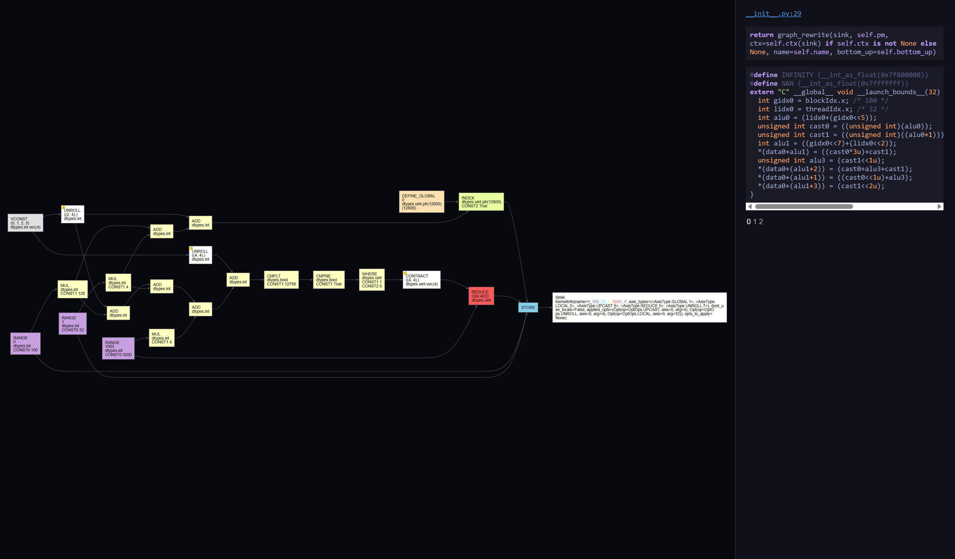
Screenshot of the Tinygrad's compute graph visualization tool. It shows the compute graph and the corresponding native kernel code lowered from the graph.
This allows you to apply its JIT compiler to compile the entire compute graph into native kernel code for hardware accelerators.
With the full compute graph, there are a lot of opportunities to optimize it by fusing the operations.
For example, here’s how you put the @TinyJIT decorator on a function to compile the entire compute graph into native kernel code:
@TinyJit
def mutate_step(
  combined_loss: Tensor, combined_paths: Tensor
) -> tuple[Tensor, Tensor]:
  min_loss, min_loss_index = combined_loss.topk(1, largest=False)
  min_path = combined_paths[min_loss_index].flatten()
  mutate(
      marketplace=marketplace,
      leading_path=min_path,
      jitter=lr,
  )
  return min_loss.realize(), min_path.realize()
I also appreciate that the library is very small, making it much easier to understand and extend. I enjoy using Tinygrad for machine learning and other high-performance computing tasks across platforms. This research will be way harder if I had to use PyTorch or other machine learning frameworks, as they assume training with backpropagation. You may need to build your own CUDA kernel or other hardware-specific code to run on GPUs if you want to speed up the training process.
Back to the topic: yes, I implemented the Marketplace algorithm using Tinygrad. As like most of my machine learning projects, I’ve open-sourced it here:
https://github.com/LaunchPlatform/marketplace
You should be able to find all the experiment code in the experiments folder.
Please pardon me, as some parts of the code might be slightly messier than my usual standards, since this is an experimental project, not a production one.
I used the beautiful_mnist example from Tinygrad’s examples folder as the target model to test my algorithm.
The implementation is simple: we break down each CNN layer into a multi-model class, like this:
[
  # layer0
  Spec(
    model=MultiModel(
      [
        MultiConv2d(structure[0][0], 1, 32, 5),
        Tensor.relu,
      ]
    ),
  ),
  # layer1
  Spec(
    model=MultiModel(
      [
        MultiConv2d(structure[1][0], 32, 32, 5),
        Tensor.relu,
      ]
    ),
    upstream_sampling=structure[1][1],
  ),
  # layer2
  Spec(
    model=MultiModel(
      [
        MultiBatchNorm(structure[2][0], 32),
        Tensor.max_pool2d,
      ]
    ),
    upstream_sampling=structure[2][1],
  ),
  # layer3
  Spec(
    model=MultiModel(
      [
        MultiConv2d(structure[3][0], 32, 64, 3),
        Tensor.relu,
      ]
    ),
    upstream_sampling=structure[3][1],
  ),
  # layer4
  Spec(
    model=MultiModel(
      [
        MultiConv2d(structure[4][0], 64, 64, 3),
        Tensor.relu,
      ]
    ),
    upstream_sampling=structure[4][1],
  ),
  # layer5
  Spec(
    model=MultiModel(
      [
        MultiBatchNorm(structure[5][0], 64),
        Tensor.max_pool2d,
      ]
    ),
    upstream_sampling=structure[5][1],
  ),
  # Layer6
  Spec(
    model=MultiModel(
      [lambda x: x.flatten(1), MultiLinear(structure[6][0], 576, 10)]
    ),
    upstream_sampling=structure[6][1],
  ),
]
In other words, we duplicate the same weights N times to test different vendor variants.
Here’s an example implementation of the multi-model version of Conv2D:
class MultiConv2d(MultiModelBase, nn.Conv2d):
  def __init__(
    self,
    vendor_count: int,
    in_channels: int,
    out_channels: int,
    kernel_size: int | tuple[int, ...],
    stride=1,
    padding: int | tuple[int, ...] | str = 0,
    dilation=1,
    groups=1,
    bias=True,
  ):
    super().__init__(
      in_channels=in_channels,
      out_channels=out_channels,
      kernel_size=kernel_size,
      stride=stride,
      padding=padding,
      dilation=dilation,
      groups=groups,
      bias=bias,
    )
    self.vendor_count = vendor_count
    self.weight = repeat(self.weight, vendor_count)
    if self.bias is not None:
      self.bias = repeat(self.bias, vendor_count)
We also modified the forward pass method to accept an extra index parameter, allowing switching between different weights from various vendors.
def __call__(self, i: Tensor, x: Tensor) -> Tensor:
  return x.conv2d(
    self.weight[i],
    self.bias[i] if self.bias is not None else None,
    self.groups,
    self.stride,
    self.dilation,
    self.padding,
  )
For the first layer, we feed training input data to different vendors (weights), producing an array of intermediate products. The next layer randomly selects N intermediate products from the upstream layer, tracking the vendor indices to form a tensor representing the product’s supply chain path. If it’s a full sampling, we sample all vendors outputs from the upstream layer. Here’s the simplified code for producing output for a layer:
def produce(
  model: MultiModel,
  x: Tensor,
  paths: Tensor | None = None,
  upstream_sampling: int = 0,
) -> tuple[Tensor, Tensor]:
  if paths is None:
    # first layer, no upstream sampling, just feed input to all vendors
    output_data = Tensor.stack(
        *(model(Tensor(i), x) for i in range(model.vendor_count)), dim=0
    )
    paths = Tensor.arange(model.vendor_count).unsqueeze(1)
    return output_data, paths

  if upstream_sampling == 0:
    # sample all vendors from the upstream layer
    upstream_sampling = x.shape[0]

  input_count = paths.size(0)
  input_indexes = Tensor.stack(
    *(
      Tensor.randperm(input_count)[:upstream_sampling]
      for _ in range(model.vendor_count)
    ),
    dim=0,
  )
  input_data = x[input_indexes]
  # merge different batches for the same vendor into one. not sure if this is needed, but at least it saves us
  # from calling the model multiple times and making the graph more complex
  merged_batches = input_data.reshape(input_data.shape[0], -1, *input_data.shape[3:])

  output_data = Tensor.stack(
    *(
      model(i, merged)
      for i, merged in zip(range(model.vendor_count), merged_batches)
    ),
    dim=0,
  )
  # breaking down merged batches back to individual batches
  output_data = output_data.reshape(-1, input_data.shape[2], *output_data.shape[2:])

  prev_paths = paths[input_indexes].flatten(0, 1)
  new_paths = (
    Tensor.arange(model.vendor_count)
    .unsqueeze(1)
    .repeat(1, upstream_sampling)
    .flatten()
    .unsqueeze(1)
  )
  merged_paths = prev_paths.cat(new_paths, dim=1)

  return output_data, merged_paths
After processing all layers, we obtain the final products, i.e the output logits.
We apply the loss function to identify the product with the lowest loss, then copy the weights from the leading vendors to the others, adding slight random mutations to explore further improvements.
The mutate function is responsible for copying the weights from the leading vendors to the others, adding slight random mutations to explore further improvements.
The code looks like this:
def mutate(marketplace: list[Spec], leading_path: Tensor, jitter: Tensor):
  for spec, leading_index in zip(marketplace, leading_path):
    multi_params = nn.state.get_state_dict(spec.model)
    for i in range(spec.model.vendor_count):
      for key, params in multi_params.items():
        leading_params = params[leading_index]
        params[i] = (
          leading_params
          + (i == leading_index).where(
            # Do not change the leading vendor
            Tensor(0),
            # Copy from the leading vendor and add a bit jitters
            (
              Tensor.uniform(
                  *leading_params.shape, low=-jitter, high=jitter
              )
            ),
          )
        ).realize()
That’s it. The implementation is surprisingly simple.
Learning Rate Is Critical
When experimenting with the Marketplace training algorithm, I realized that the learning rate plays a key role in successfully training a model, just as it does in backpropagation. I tested various learning rates to determine which one yields the best training performance. In addition to the learning rate, the learning rate schedule is also crucial. I need to reduce the learning rate over time to make the random adjustments smaller, allowing the model to fine-tune the final few decimal points of accuracy. Here’s a diagram showing the significant differences in performance based on various learning rates and decay schedules:

A chart with shows the accuracy of different learning rates and decay schedules. The best learning rate is 1e-3 with a 1e-04 decay schedule.

A chart with shows the loss of different learning rates and decay schedules. The best learning rate is 1e-3 with a 1e-04 decay schedule.

A chart with shows the learning rate value of different learning rates and decay schedules.
For now, I rely on a trial-and-error approach to find the optimal learning rate.
Batch Normalization Doesn’t Work Well with Marketplace
Interestingly, during training, I noticed that the accuracy of the testing dataset was fluctuating. I investigated the issue and identified the cause as the Batch Normalization layer. Since we are sampling various intermediate products, these products significantly affect the mean and variance of the Batch Normalization layer. However, most of these products are eventually discarded, rendering them as noise. During inference, Batch Normalization uses the running mean and variance, which are influenced by these noisy, discarded intermediate products. As a result, the accuracy fluctuates. To address this issue while retaining the benefits of normalization, I replaced the Batch Normalization layer with an Instance Normalization layer. This change resolved the problem effectively!

A chart shows the validation accuracy fluctuation for the Batch Normalization but not for the Instance Normalization.
Experiments as code
I used to collect metrics with TensorBoard for my machine learning experiments. But my experiment runs accumulate quickly, and I get lost figuring out which experiment is which real fast. I realized that I needed to organize my experiments better. I tried MLflow, and I absolutely love it. I highly recommend it if you’re doing any machine learning experiments. With MLflow, I can run experiments as code. Instead of manually running the training script with different parameters, I can write a script to run the training with different parameters. Here’s an example for the learning rate experiment:
exp_id = ensure_experiment("Learning Rate V2")
for batch_size in [32, 64, 128, 256, 512]:
  for lr in [1e-2, 1e-3, 1e-4]:
    for decay in [1e-3, 1e-4, 1e-5]:
      with mlflow.start_run(
        run_name=f"bs-{batch_size}-lr-{lr:.1e}-decay-{decay:.1e}",
        experiment_id=exp_id,
        log_system_metrics=True,
      ):
        marketplace = make_marketplace(PYRAMID32_HALF_UPSTREAM_STRUCTURE)
        train(
          step_count=3_000,
          batch_size=batch_size,
          initial_lr=lr,
          lr_decay_rate=decay,
          marketplace=marketplace,
        )
Since MLflow logs which commit you are currently on, you can easily reproduce the experiment by checking out the commit and running the script again. It’s a good practice to always commit your code before running an experiment so that the commit hash is always associated with the experiment.
Here’s a screenshot of the MLflow dashboard:
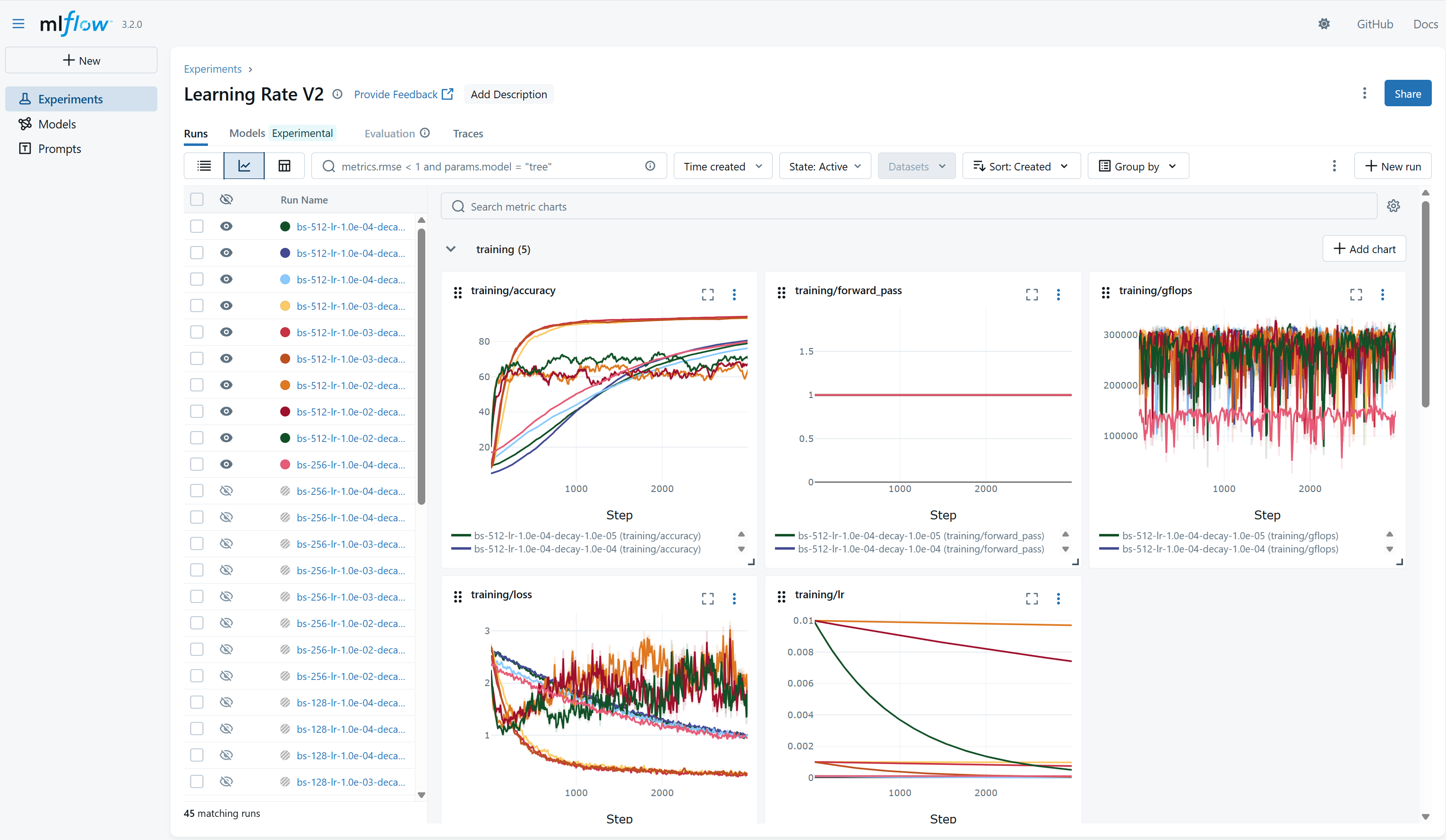
A screenshot shows the MLflow dashboard.
And with its parallel coordinates plot, you can easily see the relationship between the parameters and the performance.
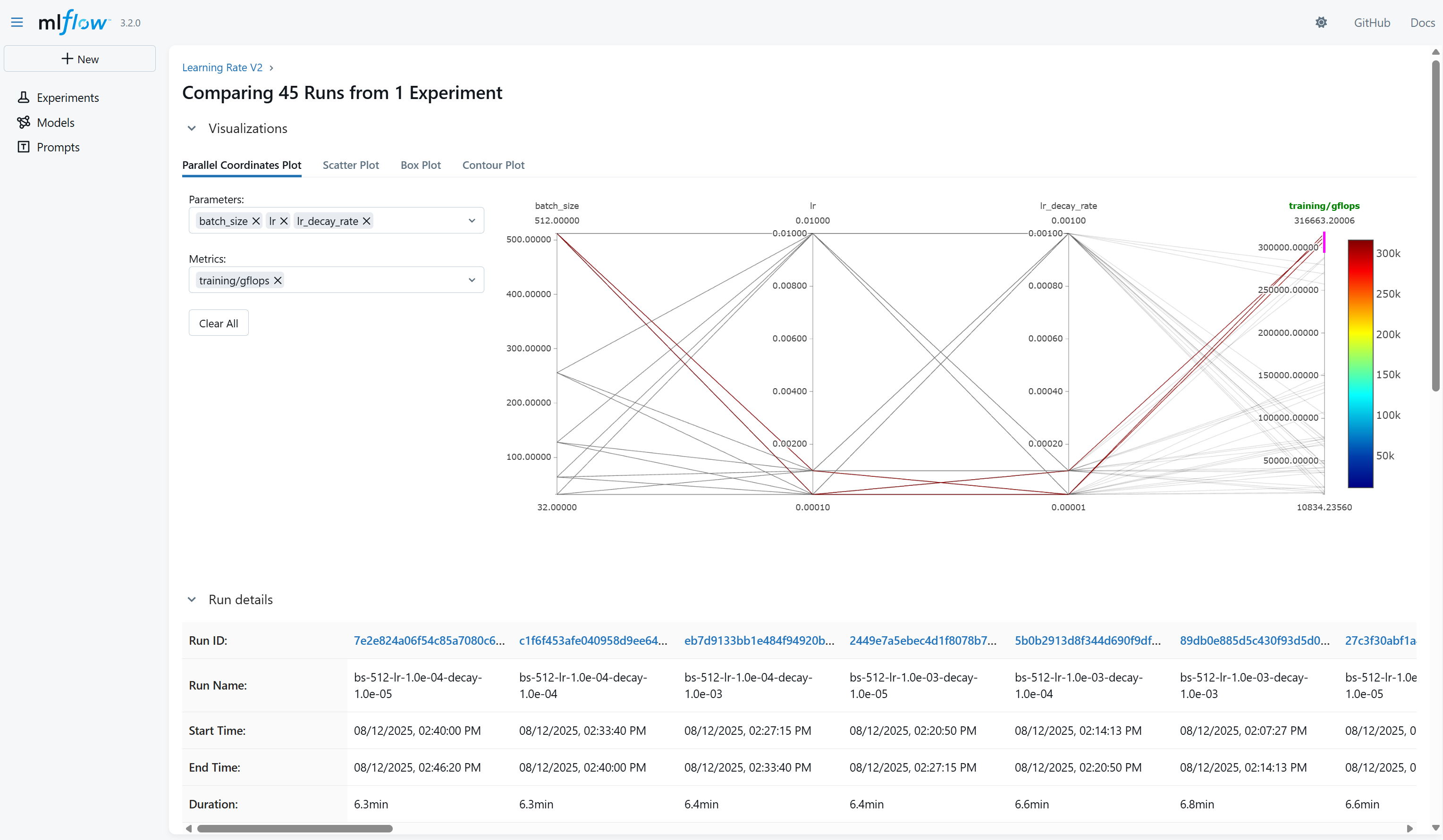
A screenshot shows the MLflow parallel coordinates plot.
The lesson I learned from this is that I should have been using MLflow all along. With the right tool, life is much easier.
Optimal Marketplace Structure
I didn’t pay much attention to the marketplace structure initially. However, I soon realized that the structure is critical. The beauty of the marketplace lies in its efficiency, as it reuses the same output multiple times. However, if the structure is poorly designed, GPU resources can be wasted on computing intermediate products that are never used. For example, with a low upstream sampling number, intermediate products in the upper layers have a lower chance of being selected downstream. Running multiple forward passes could address this, but it’s not efficient.
With full upstream sampling, all outputs from the previous layer are used. Ideally, this is what you want, as all computational results are utilized downstream. However, this approach causes the number of intermediate and final products to grow exponentially with the number of layers. Therefore, when designing the marketplace structure, we must carefully consider the number of layers.
In the MNIST CNN network, I initially assigned each Conv2D layer—and nearly every other layer—to its own specification. As a result, the marketplace had too many layers, forcing me to use an upstream sampling value to reduce the number of intermediate products. When comparing this approach to mutating all weights at once, the performance was not as poor as I expected, even with full weight mutation. This is a relatively small model, with only about 80,000 parameters. Given the limited exploration space, I concluded that having many layers in the marketplace was unnecessary. I eventually reduced the depth of the marketplace to three with full upstream sampling.
Comparison of Mutating All Weights at Once vs. the Marketplace Approach
A much simpler approach compared to the Marketplace approach is to mutate all weights simultaneously (the all-at-once approach). We can mathematically prove that the Marketplace approach is more efficient and quantify the gain from the all-at-once approach.
Consider a model with \(N\) specifications, referred to as market depth. Each specification has \(M\) vendors, representing different weight configurations. Let \(S_i\) denote the computation cost of the forward pass for specification \(i\) (where \(i = 0, 1, \dots, N-1\)).
All-at-Once Approach
In the all-at-once approach, we evaluate \(M\) different weight configurations across all \(N\) specifications. The total computation cost \(C_A\) is:
\[C_A = M \times \sum_{i=0}^{N-1} S_i\]This yields \(M\) unique final products. The unit cost per product, \(U_A\), is:
\[U_A = \frac{C_A}{M} = \sum_{i=0}^{N-1} S_i\]Marketplace Approach
In the Marketplace approach, we use full upstream sampling, processing intermediate outputs sequentially across specifications. For the first specification, we feed the input to all \(M\) vendors, with a cost of:
\[C_{S_0} = M \times S_0\]This produces \(M\) intermediate outputs. For the second specification, each of these \(M\) outputs is processed by all \(M\) vendors, yielding a cost of:
\[C_{S_1} = M^2 \times S_1\]For the third specification, the cost is:
\[C_{S_2} = M^3 \times S_2\]And so on. The total computation cost \(C_M\) is:
\[C_M = \sum_{i=0}^{N-1} M^{i+1} \times S_i\]This produces \(M^N\) distinct final products. The unit cost per product, \(U_M\), is:
\[U_M = \frac{C_M}{M^N} = \sum_{i=0}^{N-1} \frac{M^{i+1} S_i}{M^N} = \sum_{i=0}^{N-1} \frac{S_i}{M^{N-i-1}}\]Efficiency Comparison
The unit cost \(U_M\) is significantly lower than \(U_A\), especially for large \(M\) or \(N\). To quantify this, assume \(S_i = S\) (constant cost per specification). For the all-at-once approach:
\[C_A = M \times N \times S, \quad U_A = N \times S\]For the Marketplace approach:
\[C_M = S \times \sum_{i=0}^{N-1} M^{i+1} = S \times M \times \frac{M^N - 1}{M - 1}\] \[U_M = \frac{C_M}{M^N} = S \times \frac{M}{M - 1} \times \frac{M^N - 1}{M^N}\]For large \(M\), \(\frac{M^N - 1}{M^N} \approx 1\) and \(\frac{M}{M - 1} \approx 1\), so:
\[U_M \approx S\]The efficiency ratio is:
\[\frac{U_M}{U_A} \approx \frac{S}{N \times S} = \frac{1}{N}\]Thus, the Marketplace approach is approximately \(N\) times more efficient when \(M\) is large and \(S_i = S\). For non-constant \(S_i\), the efficiency depends on the distribution of \(S_i\), but the scaling factors \(M^{N-i-1}\) ensure \(U_M \ll U_A\) for \(M > 1\).
Ideally, a larger \(N\) increases efficiency, as the unit cost scales inversely with \(N\). However, the exponential growth in product count (\(M^N\)) limits scalability in practice. The vendor count \(M\) has a some impact but diminishes beyond a threshold.
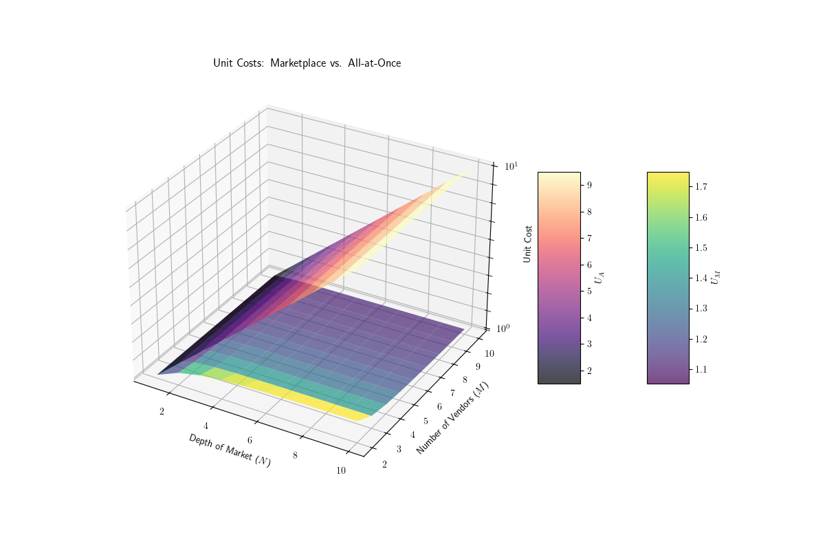
A 3D chart shows the relationship between N, M, and the per unit cost comparison between the Marketplace and the all-at-once approach. The x-axis is the depth of the marketplace, the y-axis is the number of vendors per specification, and the z-axis is the per unit cost comparison.
In the context of GPUs, compute resources are relatively inexpensive. With many cores running in parallel, a significant portion often remains underutilized. However, memory is a scarcer resource, as model weights consume substantial memory. We have established that the computational cost of the Marketplace approach is significantly lower than that of the all-at-once approach. But what about memory costs? The memory unit cost is similar, as the all-at-once approach requires \(N\) times the memory of the Marketplace approach.
Benchmarking the Marketplace Approach
With the mathematical proof, we now know that the Marketplace approach is more efficient than the all-at-once approach. With lower computational and memory costs, the same computing resources can be used to explore a larger weight space. Another benefit is that the Marketplace approach allows partial mutation of the weights. Since the previous leading vendor continues to participate in the next round, permutations of the weights can be made by changing only the downstream weights from the previous leading vendor. This helps stabilize the training process in the later stages of training. Given these theoretical benefits, let’s benchmark the Marketplace approach against the all-at-once approach.
The all-at-once approach is, in fact, a special case of the Marketplace approach, where the market depth is 1. Here is the specification for the all-at-once approach:
[
  Spec(
    model=MultiModel(
      [
        MultiConv2d(vendor_count, 1, 32, 5),
        Tensor.relu,
        MultiConv2d(vendor_count, 32, 32, 5),
        Tensor.relu,
        MultiInstanceNorm(vendor_count, 32),
        Tensor.max_pool2d,
        MultiConv2d(vendor_count, 32, 64, 3),
        Tensor.relu,
        MultiConv2d(vendor_count, 64, 64, 3),
        Tensor.relu,
        MultiInstanceNorm(vendor_count, 64),
        Tensor.max_pool2d,
        lambda x: x.flatten(1),
        MultiLinear(vendor_count, 576, 10),
      ]
    ),
  ),
]
As you can imagine, given the vendor_count value, we are essentially duplicating the same model vendor_count times.
On the other hand, the Marketplace approach was designed with three specifications, each supporting vendor_count vendors.
[
  Spec(
    model=MultiModel(
      [
        MultiConv2d(vendor_count, 1, 32, 5),
        Tensor.relu,
        MultiConv2d(vendor_count, 32, 32, 5),
        Tensor.relu,
        MultiInstanceNorm(vendor_count, 32),
        Tensor.max_pool2d,
      ]
    )
  ),
  Spec(
    model=MultiModel(
      [
        MultiConv2d(vendor_count, 32, 64, 3),
        Tensor.relu,
        MultiConv2d(vendor_count, 64, 64, 3),
        Tensor.relu,
        MultiInstanceNorm(vendor_count, 64),
        Tensor.max_pool2d,
        lambda x: x.flatten(1),
      ]
    ),
  ),
  Spec(
    model=MultiModel([MultiLinear(vendor_count, 576, 10)]),
  ),
]
Let’s try a few different configurations, and see how the training performance changes.
- Market depth: \(1\), vendor count: \(8\), final product count: \(8\)
- Market depth: \(1\), vendor count: \(16\), final product count: \(16\)
- Market depth: \(1\), vendor count: \(32\), final product count: \(32\)
- Market depth: \(1\), vendor count: \(64\), final product count: \(64\)
- Market depth: \(3\), vendor count: \(8\), final product count: \(8^3=512\)
- Market depth: \(3\), vendor count: \(16\), final product count: \(16^3=4096\)
And here’s the result:

A chart shows the accuracy of different market depth and vendor count configurations with 50% smoothing. The x-axis is the step count, and the y-axis is the accuracy. The best accuracy is achieved with a market depth of 3 and a vendor count of 16. Followed by market depth of 3 and vendor count of 8 then other all-at-once configurations.

A chart shows the loss of different market depth and vendor count configurations with 50% smoothing. The x-axis is the step count, and the y-axis is the loss at log scale. The best loss is achieved with a market depth of 3 and a vendor count of 16. Followed by market depth of 3 and vendor count of 8 then other all-at-once configurations.
As you can see, a market depth of 3 with a vendor count of 16 outperforms the all-at-once approach with a vendor count of 64. Even the market depth of 3 with a vendor count of 8 outperforms the all-at-once approach with a vendor count of 64! This demonstrates that the Marketplace approach is more efficient than the all-at-once approach. It is capable of exploring a larger weight space with the same computational resources.
Comparison with Backpropagation
Some of you may ask, what about the performance of the Marketplace approach compared to backpropagation? I am curious about the performance of the Marketplace approach compared to backpropagation as you are. To make the comparsion, I took the beautiful_mnist example code from the Tinygrad repo. As mentioned in the previous section, because the Batch Normalization layers don’t work well with the Marketplace approach, I replaced them with Instance Normalization. And for the Marketplace approach, it’s a three level deep marketplace with 16 vendors per specification, batch size is 512 and initial learning rate is 1e-3 with a 1e-04 decay schedule. Here’s the result:

A chart shows the accuracy of the Marketplace approach and backpropagation. The x-axis is the step count, and the y-axis is the accuracy. The backpropagation reaches 98% accuracy in 70 steps, while the Marketplace approach reaches 90% accuracy in 629 steps and 95% accuracy in 2.3K steps.

A chart shows the loss of the Marketplace approach and backpropagation. The x-axis is the step count, and the y-axis is the loss at log scale.
Well, not surprisingly, backpropagation is way better in this case. I didn’t expect my newborn training algorithm to beat a state-of-the-art method backed by decades of research. As you can see from the chart, it takes only 70 steps to reach 98% accuracy, while the Marketplace approach takes 629 steps to reach 90% accuracy with the same batch size. And it takes raound 2.3K steps to reach around 95% accuracy. Then it takes longer time to increase the accuracy slowly over time. With 3,000 steps, the Marketplace approach reaches 96% accuracy eventually.
Strengths of the Marketplace
As you can see, backpropagation outperforms the Marketplace algorithm. However, as engineers, it’s always about the trade-offs. Surely backpropagation is better in this case, but there are still some strengths of the Marketplace approach. Here, I list some key strengths of the Marketplace:
Scalability
The Marketplace approach has a potential advantage in scalability. Scaling backpropagation with additional GPUs is challenging because its forward and backward passes are tightly coupled, and the backward pass requires strict sequential propagation, making parallelization difficult. In contrast, the Marketplace approach is inherently scalable. In theory, there is no limit to the number of vendors you can run within the same layer, as each can independently generate a variant of the current leading vendor by “rolling the dice.” However, with more vendors, you may need to increase upstream sampling in downstream layers to evaluate them more thoroughly; otherwise, you risk wasting computational resources if intermediate products are underutilized.
Some may ask: how do you synchronize vendor weights across nodes when scaling out? Since the current approach generates random weight deltas based on the learning rate and applies them to the leading vendor’s weights, we can use a random seed value to deterministically generate these deltas. By sharing the seed across nodes, we can reconstruct the weights using the same deterministic random number generator.
The Marketplace approach can be scaled along different axes. With more vendors, you can run additional vendor variants in parallel. However, more vendors do not necessarily improve mutation quality, as a limited batch size can constrain mutation quality. Another interesting approach is to run the same set of vendor variants across multiple nodes for different batches simultaneously. It may not be necessary to process numerous batches in the early stages of training. In the later stages, to optimize the final decimal points of the loss, you may need to process many batches. I tested a bit whether we could run the same set of vendor variants across multiple nodes for different batches simultaneously to improve the training speed. I simulated the training process with multiple instances by running multiple forward passes sequentially. Counterintuitively, performance degraded with more forward passes. I am still investigating the reason. If it’s possible to scale on the dataset axis in parallel, it would be a significant improvement.
I wonder if we can scale the Marketplace approach efficiently, is it possible to shorten the training time? Like, for example, the LLM pre-training process takes 6 months, with abundant GPUs, can we shorten it to 6 weeks? I think it’s possible, but still requires a lot of research. 🤔
Optimizing the Forward Pass Enhances Training
With backpropagation, the computational graph for training differs significantly from the forward pass. Typically, to deploy a model in production, people optimize the forward pass, sometimes even building Application-Specific Integrated Circuits (ASICs) to accelerate applications like large language model (LLM) services. The Marketplace relies solely on the forward pass, so optimizing the forward pass has potential to improve the training process. It would be interesting to consider the idea of building a hardware accelerator for both inference and training.
Better GPU Utilization
Another issue with backpropagation is that its two distinct compute graphs result in lower GPU utilization than is optimal. In contrast, when observing the GPU usage rate during Marketplace training, it’s nearly always at 100%.
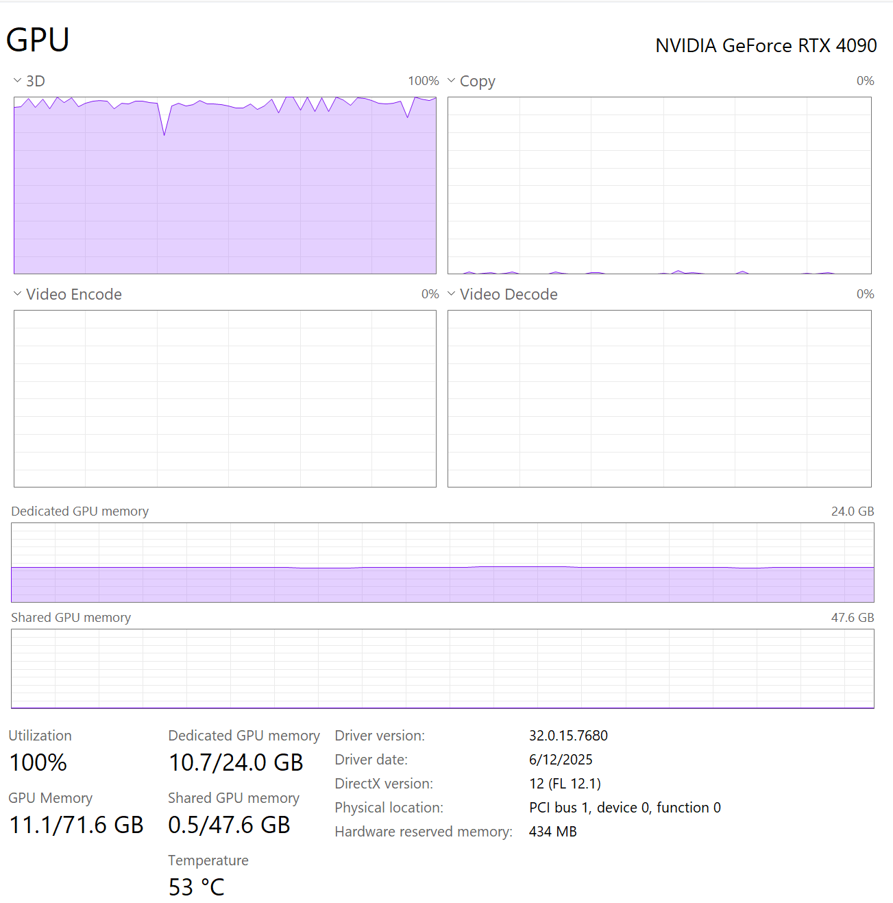
A chart shows the GPU usage rate during Marketplace training. The GPU usage rate is nearly always at 100%.
Backpropagation’s need to switch between forward and backward passes also makes it less cache-friendly. As highlighted in the previously mentioned CUDA video, GPU performance heavily depends on memory layout and access patterns. By relying solely on the forward pass, the Marketplace approach can better utilize GPUs. I heard an something funny about training with a large-scale GPU cluster: fluctuating GPU usage forced engineers to keep GPUs spinning idly to avoid sudden changes in power consumption, which placed significant strain on the power supply infrastructure. I wonder if the Marketplace could help with this by focusing on the forward pass.
No Need to Make the Model Differentiable
Another benefit of the Marketplace approach is that it doesn’t rely on computing gradients, so you don’t need to make your model differentiable. As an interesting side note, with backpropagation, some corner cases, such as ReLU, are not continuous but still function effectively. Since backpropagation has been the dominant approach for decades, I guess there has been relatively little research into non-differentiable models and their benefits. At this moment, I’m unsure of the full implications. My gut feeling suggests that for low-precision training, or even integer-based training, the Marketplace approach could be particularly beneficial. This is yet another intriguing topic for future research.
A Blockchain for Training LLMs
With the advantages of marketplace training, I can already envision some exciting applications. What’s bigger than the AI hype? How about blockchain + AI? 🤣 Seriously, though, I believe this is feasible. Here’s how I imagine it could work.
First, we need to publish the training data to make it easily accessible to all miners. An open-source dataset like Common Crawl could be used, but the specific dataset isn’t critical—the key is ensuring accessibility. We then define the training batches in a deterministic order. Each miner’s task is to find the next seeds for each layer that yield the lowest loss in combination. Miners can share their seeds on a peer-to-peer network, encapsulated with their digital signatures and public key. The miner with the lowest loss wins the mining reward. Anyone should be able to reapply the deterministic training dataset to verify whether the proposed block is indeed the best. If a branch occurs, the chain with the lowest loss prevails. This approach enables a decentralized network to pre-train an LLM on a blockchain! This sounds like an intriguing weekend project, but I’ll save it for another time. 😅
Future Research
Now that we know the Marketplace algorithm can search for optimal neural network weights on a GPU, here are some ideas for future exploration. But there are still some challenges to overcome.
Memory Efficiency
Currently, we store each vendor’s full weights, enabling parallel computation of layers with different inputs, which is highly GPU-efficient. However, this approach consumes valuable GPU memory. To explore a larger weight space with more vendor variants, we could implement seed-based random number generation for each vendor’s weights as mentioned in the previous section. This way, we can store only the seeds, freeing up GPU memory while testing N vendor variants without losing the weights.
Distributed Training
With deterministic seed-based random number generation in place, we could build a cluster to efficiently share seeds across nodes. Each node could reconstruct weights with minimal bandwidth requirements and independently run vendor variants. The only significant data transfer between nodes would likely be the intermediate products, especially if we allow cross-node upstream sampling of products.
Improved Random Weight Generation: Momentum
Currently, weight deltas are generated randomly, but the best-performing deltas contain valuable information. If a CNN filter consistently moves in a specific direction that yields good results, that direction may be worth pursuing. Introducing a momentum concept, similar to many optimizers, such as Adam, could be a valid approach to accelerate training. For example, if a direction proves effective multiple times, we could bias random weight updates toward that direction to speed up convergence. I envision that the improvement in the delta generator doesn’t need to be substantial. A slight enhancement, combined with vendor scaling, could lead to significant performance improvements.
Sub-Optimal or Bad Final Products Are Still Valuable
The current approach only keeps the best final product and its delta. But what about the others? While they don’t perform as well as the best final product and their corresponding vendor deltas, they still contain valuable information. With enough delta permutations and their corresponding final products, is it possible to statistically attribute which parameter in a big chunk of delta is responsible for a better final product? For example, we could take the loss generated from the final products and attribute it to the delta that generated each final product. By merging the delta, weighted by the attributions from the loss, we might be able to compose a better overall delta that accounts for both good and bad outcomes. I think this is yet another very interesting idea to explore.
Training Larger and Diverse Models
The Marketplace algorithm performs well with the small MNIST CNN, but its scalability remains untested. How effectively does it handle larger models? Beyond CNNs, can it be applied to other architectures, such as transformers? I’m interested in pre-training a large language model (LLM) with this algorithm to evaluate its performance and scalability. I see no particular reason why it wouldn’t work. Maybe it just takes longer to train, but I hope to scale out to compensate for the time. In fact, I’ve already trained a larger model, ResNet-18 (approximately 11 million parameters), using the Marketplace approach on a scaled MNIST dataset with limited steps. The results seem promising, though I didn’t run the experiment for long. It was a quick test, and I didn’t optimize the code.

A chart shows the accuracy of the Marketplace approach on the scaled MNIST dataset with 100% smoothing. The x-axis is the step count, and the y-axis is the accuracy. With limited steps, the accuracy is trending up steadily showing progress of the training.

A chart shows the loss of the Marketplace approach on the scaled MNIST dataset with 100% smoothing. The x-axis is the step count, and the y-axis is the loss at log scale. With limited steps, the loss is trending down steadily showing progress of the training.
With a larger model, each specification has more parameters to mutate, meaning a larger space to explore. However, we could address this by breaking it down into smaller specifications or using a larger batch size to explore the space more effectively. Another interesting idea is to shift the focus to different layers over time.
Focused Mutation
During the experiments, I forgot to remove a flag that prevents a layer from mutating. Surprisingly, this led to improved training performance. My hypothesis is that freezing some layers reduces the search space while maintaining the same capacity, allowing better focus on optimizing the remaining layers and thus improving training performance. I wonder if it makes sense to train only a few layers at a time for very large and deep models. Strategically switching focus to a few layers with large-scale vendor variants could simplify training. For example, if the first layer is a convolutional layer and the second is a fully connected layer, we could focus on training the first layer for a while, then switch to the second. In a CNN, the initial layers extract basic features, while later layers capture more complex features. Assuming the basic feature layers are sufficiently trained, their filters may not change much. If this assumption holds, we could focus more on the later layers in the later stages of training. This is another intriguing idea to test.
Optimizing the Performance of the Marketplace
Currently, I’ve implemented the Marketplace algorithm using simple Tinygrad code. I haven’t invested much effort in optimizing the code, but I believe there are many opportunities to improve performance. For example, we could maximize GPU utilization or optimize memory usage by analyzing memory patterns and making them cache-friendly. Alternatively, writing custom CUDA kernels could further enhance performance. I’m unsure if I’ll have time to pursue these optimizations, but they are worth exploring.
Design Models for the Marketplace
So far, all the models we have explored are designed for training with backpropagation. There are many factors to consider when designing models for backpropagation. For example, the model must be differentiable, and the initial weights need to be carefully chosen to avoid exploding gradients. We also use skip connections to mitigate vanishing gradients. Additionally, numerous techniques exist to enhance the training process specifically for backpropagation. But what about the Marketplace approach? What if we design a model optimized for the Marketplace approach, specifically tailored for distributing computation across multiple GPUs and nodes? This is yet another fascinating topic to explore.
Combining the Marketplace Approach with Backpropagation
I wonder if we can combine the Marketplace approach with backpropagation to train the same model in different scenarios. For example, if backpropagation gets trapped in a local minimum, can we switch to the Marketplace approach to escape it? Alternatively, could we alternate between the Marketplace approach and backpropagation at different stages of training to enhance the process? Before we can answer these questions, we need to understand the nature of the Marketplace approach. There are already so many intriguing questions to explore.
Final Thoughts
That’s it! I learned a lot from this project. Regardless if people find my research side project interesting or not, it was a fun ride for myself. It was a great exercise to think about optimizing the training process and designing an algorithm for GPU efficiency. Now I have more confidence to think about algorithms from the lens of GPU efficiency. There could be more interesting ideas to explore with GPUs.
I believe this is the best time to be alive. People from ten years ago could hardly have imagined that we’d have abundant supercomputers in our homes. With modern hardware, it’s incredible that I can conduct end-to-end experiments on my own in such a short time. We’re entering a new era of personal supercomputing. I hope you enjoyed reading about my Marketplace algorithm. Please leave a comment with any feedback or questions.